RPn is thee set of lines through the origin in Rn+1. If x=0, x defines a line through origin. If y∈Rn+1 defines the same line if y=ax,a=0. Define this as equivalence relation ∼. Then RPn=(Rn+1−{0})/∼. The x0,…,xn are homogeneous coordinates, take coordinate neighbourhood Ui={x∣xi=0}, and introduce inhomogeneous coordinate ξ(i)j=xixj, ξ(i)=ξ(i)j,(j∈{0,…,n}−{i}).
Grassmann manifold is the generalization of RPn. Define Gk,n(R) be the set of k-dimensional planes in Rn. Note that G1,n+1(R)=RPn.
Let the set of k×n matrices of rank k(k≤n) be Mk,n(R). Take A∈Mk,n(R), the k vectors ai in Rn is defined by ai=Aij. The k vectors are linearly independent and spans a k-dimensional plane.
There are infinitely many matrices that yield the same k-plane. Take g∈GL(k,R), consider Aˉ=gA∈Mk,n(R). Aˉ defines the same k-plane as A with basis changed. This defines a equivalence relation ∼: Aˉ∼A iff ∃g∈GL(k,R),Aˉ=gA. So we identify Gk,n(R) with Mk,n(R)/GL(k,R). Let A1,…,Al be all l=(kn) minors of A. Since rankA=k, there must exist α such that detAα=0. Suppose α=1 for simplicity, denote this coordinate neighborhood by U1. Then rewrite A as (A1,A~1), where A~1 is k×(n−k) matrix. Then select representative as A1−1A=(Ik,A1−1A~1). There must exist A1−1 due to A1 is full rank. Then we know that atlas U1 of Gk,n(R) is homeomorphic to Rk(n−k), dimGk,n(R)=k(n−k). In the case detAα=0, where Aα is composed columns (i1,…,ik), Aα−1A are unit vectors at column i1,…,ik. This subset of Mk,n(R) is denoted by Uα.
Product manifold: If M1={(Ui,φi)} and M2={(Uj,φj)}, M1×M2={(Ui×Uj),(φi,ψj)}, and has coordinate function (p∈M,q∈N)→(φi(p),ψj(q))∈Rm+n
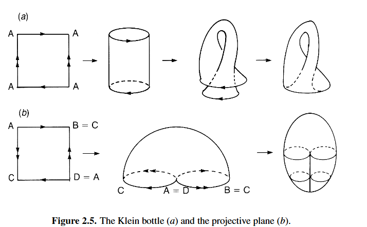
Torus T2=S1×S1, and Tn=nS1×⋯×S1
5.2.2 Vectors
To define a tangent vector we need a curve c:(a,b)→M and a function f:M→R. The f(c(t)):(a,b)→R is a 1d function, its change rate is
dtdf(c(t))t=0=∂xμ∂fdtdxμ(c(t))t=0
This defines the vector X=Xμ(∂xμ∂) and its effect on f: X[f]=Xμ∂xμ∂f. All tangent vectors in point p∈M forms the tangent space of M at p, denoted by TpM.
The cotangent space Tp∗M={ω∣ω:TpM→R}. The simplest case is df for f∈F(M), with df(V)=V(f)=Vμ∂xμ∂f∈R. Tensors T=⊗qTp∗M⊗rTpM.
5.2.6 Induced maps
A smooth map f:M→N induces a map f∗:TpM→Tf(p)N: (f∗V)[g]≡V[g∘f], and it also induces a pullback f∗:Tf(p)∗N→Tp∗M: ⟨f∗ω,V⟩≡⟨ω,f∗V⟩
5.3 Flows and Lie derivatives
The integral curve σ(t,x0) of a vector X which passes a point x0 at t=0 is a flow generated by X, if dtdσμ(t,x0)=Xμ(σ(t,x0)) with initial condition σμ(0,x0)=x0μ. The flow σ(t,x) is a diffeomorphism from M to M for fixed t∈R, and is a commutative group: σt∘σs(x)=σt+s(x), σ0=I, σ−t=σt−1, so for infinitesimal ϵ, σϵμ(x)=σμ(ϵ,x)=xμ+ϵXμ(x)
Note that σ−ϵ generates a map (σ−ϵ)∗:Tσϵ(x)M→TxM, so we can move Y∣σϵ(x) to Y∣x and differentiate them: the Lie derivative is defined as LXY=limϵ→0ϵ1[(σ−ϵ)∗Y∣σϵ(x)−Y∣x], where σ is the flow of X.
So LXY=(Xμ∂μYν−Yμ∂μXν)eν. define [X,Y] by [X,Y]f=X[Y[f]]−Y[X[f]], so LXY=[X,Y]
Geometrically, the Lie bracket shows the non-commutativity of two flows. Consider two flow σ(s,x),τ(t,x) generated by vector fields X,Y, if we first move ϵ along flow σ then move δ along τ, we get the coordinate
Define the exterior product of a q-form and an r-form ∧:Ωpr(M)×Ωpr(M)→Ωpq+r(M) by a trivial extension. Let ω∈Ωpq(M) and ξ∈Ωpr(M), for example. The action of the (q+r)-form ω∧ξ on q+r vectors is defined by
We find that LXω=(diX+iXd)ω. This is also true for a general r-form.
Let X,Y∈X(M) and ω∈Ωr(M). Show that
i[X,Y]ω=X(iYω)−Y(iXω)
and iX is an anti-derivation:
iX(ω∧η)=iXω∧η+(−)rω∧iXη
and nilptent: iX2=0. Use the nilpotency to prove
LXiXω=iXLXω
Reformulate Hamiltonian mechanics in terms of differential forms: Let H be hamiltonian and (qμ,pμ) be its phase space.
Define 2-form ω=dpμ∧dqμ, called symplectic two-form.
Itroduce a one-form θ=qμdpμ then ω=dθ. Given a function f(p,q) in phase space, define Hamiltonian vector field
Xf=∂pμ∂f∂qμ∂−∂qμ∂f∂pμ∂
Easy to verify:
iXfω=−∂pμ∂fdpμ−∂qμ∂fdqμ=−df
Let f=H, XH is vector field generated by Hamiltonian function, we obtain from Hamiltonian eq. of motion
dtdqμ=∂pμ∂H,dtdpμ=−∂qμ∂H
XH=dtd
The symplectic 2-form ω is invariant along the flow generated by XH:
LXHω=d(iXHω)+iXH(dω)=d(iXHω)=−d2H=0
Conversely if X satisfies LXω=0, ∃H such that Hamilton's eq of motion is satisfied along the flow generated by X. This follows from previos observation that LXω=d(iXω)=0, so ∃H s.t. iXω=−dH.
iXf(iXgω)=−iXf(dg)=[f,g]PB
5.5. Integration of differential forms
For an orientable manifold, take a volume element ω. Function f:M→R has integration over neiborhood Ui defined by an m-form fω:
∫Uifω=∫φ(Ui)f(φi−1(x))h(φi−1(x))dx1…dxm
Once the integral of f over Ui is defined, the integral over whole M is given with the help of the partition of unity defined now:
Take an open covering {Ui} of M such that each point of M is covered with a finite number of Ui. If a family of differentiable functions satisfies
0≤ϵi(p)≤1
ϵi(p)=0 if p∈/Ui and
ϵ1(p)+⋯=1 for any point p∈M the family {ϵ(p)} is called a partition of unity subordinate to the covering {Ui}.
It follows that f(p)=∑if(p)ϵi(p)=∑ifi(p), then we maydefine the integral by
∫Mfω=i∑∫Uifiω
e.g. atlas of S1 is U1=S1−{(1,0)} and U2=S1−{(−1,0)}. ϵ1(θ)=sin22θ and ϵ2(θ)=cos22θ is a partition of unity subordinate to {Ui}. Let us integrate a function f=cos2θ.
We have left h arbitrary provided it is strictly positive so far. h is multiplied by Jacobian under change of coordinates, there is no canonical way to single out the component h; h=1 in one coordinate might not imply h=1 in other. The situation changes if the manifold is endowed with a metric.
5.6. Lie groups and Lie algebra
5.6.2 Lie algebras
Left and right translation of g∈G by a is defined by
Rag=ga,Lag=ag
they are diffeomorphisms from G to G. Vector field X on a Lie group G is left-invariant vector field if La∗X∣g=X∣ag
A vector V∈TeG defines a unique left-invariant vector field XV throughout G by
XV∣g=Lg∗V,g∈G
because XV∣ag=Lag∗V=(LaLg)∗V=La∗Lg∗V=La∗XV∣g. Conversely a left-invariant vector field X defines a unique vector V=X∣e∈TeG. Denote the set of left-invariant vector fields g.
We show that g is closed under Lie bracket: Take two points g,ag=Lag, apply La∗ to Lie bracket [X,Y] of X,Y∈g, we have
La∗[X,Y]∣g=[La∗X∣g,La∗Y∣g]=[X,Y]∣ag
where left invariances of X,Y have been used. thus [X,Y]∈g.
GL(n,R) have n2 entries xij as its coordinates. The unit element e=In=δij. Let g={xij(g)}, a={xij(a)} be elements of GL(n,R). The left translation is Lag=ag=∑kxik(a)xkj(g). Take a vector V=∑Vij∂xij∂∣e∈TeG where Vij are the entries of V. The left-invariant vector field generated by V is
The gV is the usual matrix multiplication of g and V. The vector XV∣g is often abbreviated as gV since it gives the components of the vector.
The Lie bracket of XV and XW generated by V=Vij∂xij∂∣e and W=Wij∂xij∂∣e is
[XV,XW]∣g=∑(g[V,W])ij∂xij∂g
These relations remain true for any matrix group, we establish that
Lg∗V=gV,[XV,XW]∣g=Lg∗[V,W]=g[V,W]
The set of left-invariant vector fields g with Lie bracket [⋅,⋅]:g×g→g is called the Lie algebra of a Lie group G.
5.6.3 The one-parameter subgroup
5.6.4 Frames and structure equation
Let the set of n vectors {V1,V2,…,Vn} be a basis of TeG where n=dimG. The basis defines the set of n linearly independent left-invariant vector fields {X1,…,Xn} at each point G defined by Xμ∣g=Lg∗Vμ. Since [Xμ,Xν]∣g is again an element of g, it can be expanded in terms of {Xμ} as
[Xμ,Xν]=cμνλXλ
where cμνλ are structure constants of Lie group G. If G is matrix group, the LHS at g=e is precisely the commutator of matrices Vμ and Vν; We may show that structure constants are indeed constants independent of g. Acting Lg∗ to Lie bracket,
[Xμ,Xν]∣g=cμνλ(e)Xλ∣g
which shows the g-independence. The structure constants determine a Lie group completely in a sense.
Define the canonical one-form or Maurer-Cartan form on Gθ:TgG→TeG by
θ:X↦(Lg−1∗)X=(Lg)∗−1X,X∈TgG
The canonical one-form θ can be expanded as θ=Vμ⊗θμ, where {Vμ} is the basis of TeG, {θμ} is the dual basis Te∗G .
The canonical one-form satisfies
dθ+21[θ∧θ]=0
where dθ≡Vμ⊗dθμ,[θ∧θ]≡[Vμ,Vν]⊗θμ∧θν
5.7 The action of Lie groups on manifolds
Lie groups often appears as transformations acting on a manifold, e.g. SO(3) is the rotations in R3, Poincare group is the set of transformations acting on Minkowski spacetime.
Let G be a Lie group and M a manifold. The action of G on M is a differentiable map σ:G×M→M which satisfies
σ(e,p)=p,∀p∈M
σ(g1,σ(g2,p))=σ(g1g2,p) We often use gp notation for σ(g,p)
examples: SL(2,C) can be mapped to O(1,3): A∈SL(2,C),x∈M4,Ax:=AX(x)A†=X(Ox),O∈O(1,3), where xμ=21Tr(σμX), σμ=(I,X,Y,Z). Note A and −A gives the same element of O(1,3).
A=exp[−i2θ(n⋅σ)]=cos2θI2−i(n⋅σ)sin2θ
is mapped to rotation about n by angle θ, i.e. O(3) subgroup of O(1,3). A(θ+2π)=−A(θ) in SL(2,C) but they map to same element in O(3). The boost along n^ with v=tanhα is
A=exp[2α(n⋅σ)]
In fact, this map is an one-to-one correspondence from SL(2,C) to O+↑(1,3)={Λ∈O(1,3)∣detΛ=1,Λ00>0}
The action σ is said to be
transitive if ∀p1,p2∈M, ∃g∈G, σ(g,p1)=p2
free if ∀g=e has no fixed points in M; in other words, if ∃p∈M such taht σ(g,p)=p, g=e.
effective if the unit element e∈G is the unique element that defines the trivial action on M, i.e. if σ(g,p)=p for all p∈M, then g must be unit element e.
5.7.2 Orbits, isotropy groups
The orbit of p under action σ is defined by
Gp={σ(g,p)∣g∈G}
If the action is transitive the orbit of any p∈M is M.
The isotropy group of p∈M is a subgroup of G defined by
H(p)={g∈G∣σ(g,p)=p}
which is also called little group or stabilizer group of p.
Let G be a Lie group acting on M transitively and H(p) be an isotropy group of p∈M. H(p) is a Lie subgroup and the coset space G/H(p) is a homogeneous space. If they satisfy certain requirements, G/H(p) is homeomorphic to M.
Let G=SO(3) acting on R3, H=SO(2) be the isotropy group of x∈R3. SO(3) acts on S2 transitively and we have SO(3)/SO(2)≅S2. Since SO(2) is not normal subgroup of SO(3), S2 doesnot admit group structure. Generalize:
SO(n+1)/SO(n)=Sn
O(n+1)/O(n)=Sn since O(n+1) acts on Sn transitively
U(n+1)/U(n)=SU(n+1)/SU(n)=S2n+1
O(n+1) acts on Rn+1. If in RPn, x∼x′ and g∈O(n+1), gx∼gx′, which induces an action on RPn. Clearly this is transitive. If we take p in RPn which corresponds to (1,0,…,0)∈Rn+1, the isometry group is
H(p)=(±100O(n))=O(1)×O(n)
note O(1)=Z2={1,−1}. So
O(n+1)/[O(1)×O(n)]≅Sn/Z2≅RPn
Generalize to Grassmann manifolds: Gk,n(R)=O(n)/[O(k)×O(n−k)]
5.7.3 Induced vector fields
Define a flow in M by σ(t,x)=exp(tV)x, and define a vector field called induced vector field denoted by V♯:
V♯∣x=dtdexp(tV)xt=0
Consider SO(2) acts on M=R2. V=(01−10). First
exptV=(costsint−sintcost)
and the induce flow through x=(x,y) is
V♯∣x=−y∂x∂+x∂y∂
5.7.4 Adjoint representation
Take a∈G and define homomorphism ada:G→G by conjugation,
ada:g↦aga−1
Restrict the induced map ada∗:TgG→TadagG to g=e,
Ada:TeG→TeG
where Ada≡ada∗∣TeG. If G is a matrix group, the adjoint representation becomes a simple matrix operation. Let g∈G,XV∈g and σV(t)=exptV be one-parameter subgroup generated by V∈TeG. Then adg acting on σV(t) yields gexp(tV)g−1=exp(tgVg−1)
Leave a Comment