3 PI quantization of a Bose particle

Suppose at $t_{i}$, the particle is at $x_{i}$. The probability amplitude of finding particle at $x_{f}$ at $t_{f}$ is

$$\begin{equation} \left<x_{f},t_{f}|x_{i},t_{i}\right> \end{equation}$$

where the vectors are defined in Heisenberg picture

$$\begin{equation} \begin{aligned} \hat{x}(t_{i})\ket{x_{i},t_{i}} = x_{i}\ket{x_{i},t_{i}} , \\ \hat{x}(t_{f}) \ket{x_{f},t_{f}} = x_{f} \ket{x_{f},t_{f}} \end{aligned} \end{equation}$$

Rewrite the probability amplitude in terms of Schrodinger picture: let $\hat{x}=\hat{x}(0)$ be position operator with $\hat{x}\ket{x}=x\ket{x}$, since $\hat{x}$ has no time dependence, its eigenvector should be time independent. If

$$\begin{equation} \hat{x}(t_{i}) = e^{i \hat{H} t_{i}} \hat{x} e^{-i \hat{H} t_{i}} \end{equation}$$

is substituted, we have

$$\begin{equation} \begin{aligned} e^{i \hat{H}t_{i}}\hat{x} e^{-i \hat{H}t_{i}}\ket{x_{i},t_{i}} & = x_{i}\ket{x_{i},t_{i}} \\ \hat{x} [e^{-i \hat{H}t_{i}}\ket{x_{i},t_{i}} ] & = x_{i} [e^{-i \hat{H}t_{i}}\ket{x_{i},t_{i}} ] \end{aligned} \end{equation}$$

so $\ket{x_{i},t_{i}}=e^{iH t_{i}}\ket{x_{i}}$ and $\ket{x_{f},t_{f}}= e^{iHt_{f}}\ket{x_{f}}$, so

$$\begin{equation} \bra{x_{f},t_{f}} x_{i},t_{i}\rangle = \bra{x_{f}} e^{-i \hat{H}(t_{f}-t_{i})} \ket{x_{i}} =h(x_{f},x_{i};i(t_{f}-t_{i})) \end{equation}$$

define heat kernel of $\hat{H}$ $h(x,y;\beta)=\bra{x}e^{-H\beta}\ket{y}$.

Suppose Hamiltonian is of the form $H=\frac{p^{2}}{2m}+V(x)$

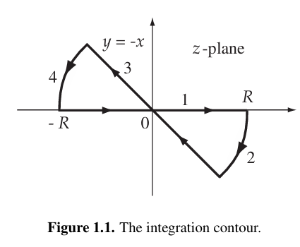
\fcolorbox{pink}{}{Lemma 1.2}
Let $a>0$. Then

$$\begin{equation} \int _{-\infty}^{\infty} \exp\left(-iap^{2} \right)\, dp = \sqrt{ \frac{\pi}{ia} } \end{equation}$$

Note: use the following contour.

\fcolorbox{pink}{}{End Lemma}

After repeating,

$$\begin{equation} \left<x_{f},t_{f}|x_{i},t_{i}\right> = \int \mathcal{D}x \exp\left[ i \int _{t_{i}}^{t_{f}} \, dt L(x,\dot{x}) \right] , L(x,\dot{x})\equiv \frac{m}{2}\dot{x}^{2} - V(x) \end{equation}$$

3 Imaginary time, partition function

Suupose $H$ is positive definite: $\mathrm{Spec} H = \{0<E_{0}\leq E_{1}\leq\dots\}$, suppose for simplicity that ground state is not degenerate. Then the spectral decomposition of $e^{-iHt}$ is given by

$$\begin{equation} e^{-iHt}=\sum_{n} e^{-iE_{n}t} \ket{n} \bra{n} \end{equation}$$

and is analytic in lower half-plane of $t$, where $H\ket{n}=E_{n}\ket{n}$. Introduce wick rotation

$$\begin{equation} t=-i\tau, \tau\in \mathbb{R}_{+} \end{equation}$$

where $\tau$ is regarded as imaginary time, which is also known as Euclidean time since $t^{2}-\vec{x}^{2}= -(\tau ^{2}+\vec{x}^{2})$.

$$\begin{equation} \begin{aligned} \dot{x}= \frac{dx}{dt}=i \frac{dx}{d\tau} \\ e^{-iHt}=e^{-H\tau} \end{aligned} \end{equation}$$

and thus

$$\begin{equation} \left<x_{f},\tau_{f}|x_{i},\tau_{i}\right> = \left<x_{f}|e^{-H (\tau_{f}-\tau_{i})}|x_{i}\right>= \int \mathcal{\bar{D}}x e^{-\int _{\tau_{i}}^{\tau_{f}} \, d\tau \left[ \left(1/2 m\right) (dx/d\tau)^{2} + V(x)\right]} \end{equation}$$

For a given Hamiltonian, the partition function is

$$\begin{equation} Z(\beta)= \mathrm{Tr} e^{-\beta H}\qquad\left(\beta>0\right) \end{equation}$$

in eigenvector basis,

$$\begin{equation} Z(\beta) = \int \, dx \left<x | e^{-\beta H}|x\right> = \int _{\text{periodic}} \mathcal{\bar{D}}x \exp \left\{ - \int _{0}^{\beta} \, d\tau \left( \frac{1}{2}m\dot{x}^{2} + V(x) \right)\right\} \end{equation}$$

Time ordered product, generating functional

$$\begin{equation} T[A(t_{1})B(t_{2})] = A(t_{1})B(t_{2})\theta(t_{1}-t_{2})+ B(t_{2})A(t_{1})\theta(t_{2}-t_{1}) \end{equation}$$

Generalization to more than 3 operators should be trivial. Operators in the bracket are rearranged so that the time parameters decrease from left to right. The $n$-operator T-product has $n!$ terms, each with $n-1$ heaviside functions.

COnsider

$$\begin{equation} \left<x_{f},t_{f}\mid T[\hat{x}(t_{1})\hat{x}(t_{2})\dots \hat{x}(t_{n})]\mid x_{i},t_{i}\right> ,\qquad \end{equation}$$

Suppose $(t_{i}<t_{1}<\dots<t_{n}<t_{f})$. Inserting completeness relation

$$\begin{equation} 1= \int _{-\infty}^{\infty} \, dx_{k} \ket{x_{k},t_{k}} \bra{x_{k},t_{k}} \end{equation}$$

,

$$\begin{equation} \begin{aligned} \left<x_{f},t_{f}| \hat{x}(t_{n})\dots \hat{x}(t_{1}) | x_{i},t_{i}\right> & =\int \, dx_{1}\dots dx_{n} x_{1}\dots x_{n} \left<x_{f},t_{f} | x_{n},t_{n}\right> \dots \left<x_{1},t_{1}| x_{i},t_{i}\right> \\ & = \int \mathcal{D}x x(t_{1}) \dots x(t_{n}) e^{iS} \end{aligned} \end{equation}$$

in the second equality we expressed each $\left<x_{k},t_{k}|x_{k-1},t_{k-1}\right>$ as path integral. Note that $\hat{x}(t_{k})$ in the LHS is a Heisenberg operator, and $x(t_{k})=x_{k}$ on the RHS is a real value of path $x(t)$.

Define generating functional $Z[J]$ to obtain the matrix elements of $T$-products efficiently. Couple $J(t)$ to coordinate $x(t)$:

$$\begin{equation} S[x(t),J(t) ] = \int _{t_{i}}^{t_{f}} \, dt \left[ \frac{1}{2}m\dot{x}^{2}-V(x)+xJ\right] \end{equation}$$

The translation amplitude in presence of $J(t)$ is denoted by $\langle x_{f},t_{f}|x_{i},t_{i}\rangle$, so

$$\begin{equation} \left<x_{f},t_{f}|T[x(t_{n})\dots x(t_{1})]|x_{i},t_{i}\right> = (-i)^{n} \frac{\delta ^{n}}{\delta J(t_{1})\dots\delta J(t_{n})} \left. \int \, \mathcal{D}x e^{iS[x(t),J(t)]} \right|_{J=0} \end{equation}$$

Suppose the system under consideration is in ground state $\ket{0}$ at $t_{i}$ and calculate probability amplitude with which the system is also in ground state at $t_{f}$. Suppose $J(t)\neq 0$ only for $[a,b] \subset [t_{i},t_{f}]$. The transition amplitude in presence of $J(t)$ may be obtained from $H^{J}=H-x(t)J(t)$ and the unitary operator $U^{J}(t_{f},t_{i})$ of Hamiltonian.

$$\begin{equation} \begin{aligned} \left<x_{f},t_{f}|x_{i},t_{i}\right> & = \left<x_{f}| U^{J}(t_{f},t_{i})|x_i\right> \\ & = \bra{x_{f}} e^{-iH(t_{f}-b)} U^{J}(b,a) e^{-iH(a-t_{i})} \ket{x_{i}} \\ & = \sum_{mn} \bra{x_{f}} e^{-iH(t_{f}-b)}\ket{m} \bra{m} U^{J}(b,a)\ket{n} \bra{n} e^{-iH(a-t_{i})} \ket{x_{i}} \\ & = e^{-iE_{m}(t_{f}-b)}e^{-iE_{n}(a-t_{i}) } \left<x_{f}|m\right> \left<n|x_{i}\right> \bra{m} U^{J}(b,a) \ket{n} \end{aligned} \end{equation}$$

where $\ket{m},\ket{n}$are energy vectors. Next rotate the time variable $t\to-i\tau$, $e^{-iEt}\to e^{-E\tau}$, then take limit $\tau_{f}\to \infty,\tau_{i}\to-\infty$, which picks up ground states $m=n=0$. Thus

$$\begin{equation} \lim_{ t_{f} \to \infty ,t_{i}\to-\infty} \left<x_{f},t_{f}|x_{i},t_{i}\right>_{J} = \left<x_{f}|0\right> \left<0|x_{i}\right>Z[J] \end{equation}$$

where we have defined generating functional $Z[J]= \bra{0} U^{J}(b,a) \ket{0} = \lim_{ t_{f} \to \infty, t_{i} \to -\infty } \bra{0}U^{J}(t_{f},t_{i})\ket{0}$, and

$$\begin{equation} Z[J] = \lim_{ t_{f} \to \infty ,t_{i}\to-\infty} \frac{\left<x_{f},t_{f}|x_{i},t_{i}\right>_{J}}{\left<x_{f}|0\right> \left<0|x_{i}\right>} \end{equation}$$

The denominator is a constant independent of $J$. Now we have PI representation of $Z[J]$:

$$\begin{equation} Z[J] = \mathcal{N} \int \mathcal{D}x\ e^{iS[x,J]} \end{equation}$$

where nomalization constant $\mathcal{N}$ is chosen so that $Z[0]=1$. $Z[J]$ generates matrix elements of $T$-product between ground states:

$$\begin{equation} \left<0| T[x(t_{1})\dots x(t_n)]|0\right> = (-i)^{n} \frac{\delta ^{n}}{\delta J(t_{1})\dots\delta J(t_{n})}Z[J] |_{J=0} \end{equation}$$

Leave a Comment

Plain Markdown

Post Comment

Markdown Preview